Showing posts with label Excel. Show all posts

Using the Switch Function to change values to text or the oposite

Easily add values of certain cells meeting certain cirteria.
Show me more...

How to Create a Gantt Chart with Progress Tracking using Excel Charts

Easily add values of certain cells meeting certain cirteria.
Show me more...

Using the SUMIF Excel Function to add desired values that match certain criteria.

Easily add values of certain cells meeting certain cirteria.
Show me more...

Excel: Delete unlocked / unprotected cells with a single keystroke

Use this method to delete all editable cells on a protected document.
Show me more...

CONCATENATE Excel Function to Create Titles from Cells

Use the CONCATENATE Function to create sentences from several Cells in Excel
Show me more...

[Guest Post] MS Excel: How to find the corresponding value for a given entry

Using the VLOOKUP function in Excel
Català - Castellano - Deutsch
Another Guest post by my brother about Excel. Imagine you have this list, where each letter has a value
Then you have a given list such as, and you want to have the value for each letter:
You just have to write the following: =Vlookup(value you want to find; matrix where the value has to be found; number of column where the value is;”false” if you want to find the exact value) In our example, this would mean you write in Sheet 2, Cell B2 the following: =vlookup(A2;Sheet1!A:B;2;FALSE) And the result would be:

Show me more...

[Guest Post] Some useful shortcuts for Excel

Some useful shortcuts for Excel. A guest post by my brother Jordi.
Català - Castellano - Deutsch
This is a guest post by my brother Jordi. A list of useful shortcuts for MS Excel that will make your workflow much faster. Here they come:
  • Ctrl+”+”: Add a new column or row. Click on the column/row where you want to add and press “Ctrl” and at the same time the “+”.
  • Ctrl+”-“: Delete a new column or row. Select the column/row want to delete and press “Ctrl” and at the same time the “-”.
  • F2: Modify a cell. When you are in a cell, press F2 and you will be able to modify directly the cell without the need to double-click it.
  • F4: Repeat an action: When you want to repeat and action you just performed, press F4 and the last action you made will be repeated.
  • F9: recalculate the values. Sometimes the excel sheet are put into manual calculation, if you want the sheet to calculate and show you the values, pres F9
  • Ctrl + “up arrow”/“down arrow”: Move to the first/last line with values: Press Ctrl + “up arrow”/“down arrow”


Show me more...

Excel: Grouping Rows or Columns

When Excel Spreadsheets become big you might want to have your cells grouped so you can easily show and hide some of them as you please.
Català - Castellano - Deutsch
We use excel sheets for wide variety of uses. When theses spreadsheets become complicated and big or even huge, having ways to show or hide parts of the sheet is critical to be able to work with them without spending half of your time scrolling up and down (or even worse, left and right). On way to do that is to group cells together. And it is very simple to do.


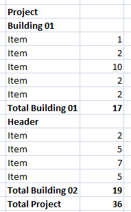
A common layout on spreadsheets is to have a header that precedes some items and even some sub-items. Something like you see on the picture above these lines. If want to be able to hide the items and only see headers and totals, we must do the following.
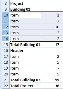
  1. Select the cells you want to group (be able to hide)
  2. Go to Data -> Group and select either Rows or Columns and click OK.
The result will be somthing like this, where Minus signs appear to the right to show you that you can hide some cells.
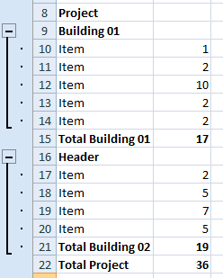
Then if you click on those minus signs, you can get something like this.


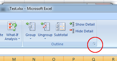
To be able to have the + / - signs on the upper part you have to go to the Layout settings and uncheck "summary rows below detail" (see images below)


Hope this helps!


Show me more...

Excel: Creating a Drop Down List with Values on a Different Sheet

Simple step by step guide on how to set up a drop down list in excel
Català - Castellano - Deutsch
In many situations we might want to have a cell in Microsoft Excel where only certain values from a list are allowed. The best way to do this is to create a drop down list with the closeable values. To do that, follow these simple steps.
  1. On a separate sheet (you can do it on the same one as well) create the list of values you want to appear in the drop down list. Put one in each cell.
  2. Drag select all those cells and enter a Name on the Name box (upper right near the formula bar). For this example we could use Listofvalues01 for example. use no spaces.
  3. Then select the cell (or multiple cells) where you want that drop down list to appear.
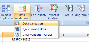
  4. With the cell or cell selected, go to the "Data" tab on the ribbon, and select Data validation -> Data Validation
  5. Go to the settings tab
  6. On "Allow" select "Lists" and check "ignore blank" and "in-cell drop down".
  7. On "Source" type =Listofvalues01 or whatever name you gave to the list of values on step 2.
  8. Click OK and go to the cell. An arrow should appear next to it and if you click on it you will see the list of closeable values
See the image below for a graphical explanation of this process.


Alternatively you could have the values on the same sheet where the drop down list appears. If you do so, you can avoid step 2, and on Step 7 instead of entering =Listofvalues01 you could simply select the cells where the list of values is (on the same sheet).

In Excel 2010, you can use this alternative method even on values being on a different sheet, but be aware that the drop down list will not work if the file is opened by a 2007 or previous version of Excel, so this option is not recommended. Either use the Namerange option (the one described in the 8 steps), or have the values in the same spreadsheet.

Show me more...

Excel: Turn numbers exported from ACAD into European Format

There is a quick way to turn numbers in Excel into European format and to remove apostrophes.
Català - Castellano - Deutsch
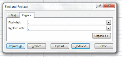
European Number Format, uses a coma as a decimal separator instead the period of the English format. When exporting data from AutoCAD to Excel using the DATAEXTRACTION command, the numbers exported are in English format, so to transform them to the European Format we need to replace the points for comas. This can very done very easy by using the find and replace function in Excel. Type CTRL + F or click the Replace button on the Editing area of the Home Tab (Excel 2007). Find Points and replace them by comas, and select Replace All.


There is an extra step needed if we want to be able to use the data from AutoCAD in Excel as numbers. All the Cells exported from CAD start with an apostrophe ('). See below.


This makes the numbers not usable as such. Luckily there is a trick to batch remove this sign. If you have a column with numbers, insert a new column to its right. On the cell next to the first number in the row enter the follwing fórmula.


Where D2 is the Cell with the numbers with the apostrophe you need to eliminate. Then copy the cell next to all numbers you want to transform. You will see now the result of the formula as the number you want to use. Something like this:


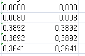
The left cell is the one still containing the apostrophes, and that is why the numbers are aligned to the left. The one on the right is the result of the formula we have applied.

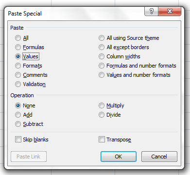
A final step I would recommend is to copy all these new cells and paste them in a new column using Paste Special. Paste Special can be accessed after copying some cells by right clicking on a cell. Then On the Paste Special Window Select "Values".


That's it, now you can delete the other columns (the one with the apostrophes and the one with the formulas, and you have just the new column with plain numbers. The explanations is long, but the process takes lest than a minute.


Show me more...

AutoCAD: Extracting Data to Excel

Do you need to extract the object properties to an excel sheet? Easy, don't do it manually.
Català - Castellano - Deutsch
Sometimes we might need to get information of some of the objects exported to an Excel Sheet to do some further calculations there. A good way to automate this process if we have a lot of objects is to use the DATAEXTRACTION wizard.
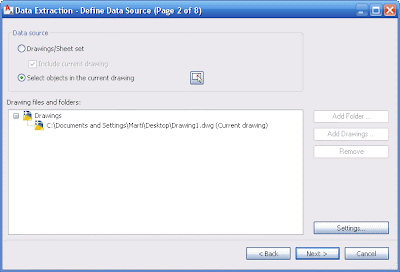
To access it simply type DATAEXTRACTION and follow the instructions. You'll be able to select which objects you want to export data from (or alternatively all the objects on a drawing or several drawings, see below)


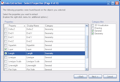
You can always select which properties of the objects you want exported (length, object type, layer, color, etc) making it simple to later differentiate the objects in Excel.


By default, Object Name and Count will also be exported. Object Count means that if you have 2 objects with their properties being identical (those that you are exporting), the exported excel sheet will only show 1 row, and a count of 2. Name, is basically the type of object. See the image with 5 lines, and the excel sheet obtained after exporting only the layer and length of the objects.


As you can see the lines with equal length and layer show only once in the table, with a count of 2. If we had included other properties in the export settings (like start X or start Y) the lines would not have been grouped because the data extracted would be different.

Show me more...

AutoCAD: Using an Excel Sheet as if it was an XREF

You can insert an Excel sheet in AutoCAD and keep it linked so when the sheet is updated, it shows the updates in AutoCAD
Català - Castellano - Deutsch
Many times, we use MS Excel (or similar)to show area charts, parking counts, unit types, etc. For a long time I had been printing the Excell Sheets to PDF format, turning them nto JPEGs and then inserting them as images in AutoCAD. BEsides being a 3 step process, it has the disadvantage that whenever the worksheet was updated, the process needed to be done again and again.
I just discovered recently that there is no need to Print as PDF and insert an Excel Sheet. It can be inserted in a way that it will remain linked and it will update. And it is much simpler than you think.
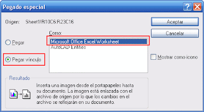
Simply select the part of the sheet you want to insert in Excel, press Ctrl + C (or Edit --> Copy). Then, go to the AutoCAD drawing you want to insert it in an go to Edit --> Paste Special. You should see a dialog like the one below.

On the left side, select "Paste Link", and from the options offered on the right side, select "Microsoft Office Excel Worksheet". That's it, almost as simple as Copy and Paste with just a few extra tweaks, and it will save you lots of time. ANytime you save the Excel Sheet it will automatically update in AutoCAD.

Show me more...